The goal of this lab is to code a minimalist finite element model in C ++. Throughout this lab, you are asked to keep a report of your implementation choices, and the algorithms you will put in place.

Download the sources with the command:

git clone https://github.com/courtecuisse/msofa.git

The goal is to complete the main functions of this code. All the functions that need to be implemented are preceded by the following comment:

/// TODO: implement this function

To be able to test the code from the beginning of the Lab, a binary version of the implemented functions is provided in the file lib/microSofaImpl.so

By default, all functions that you need to implement are declared but not implemented (commented). As soon as you uncomment any of these functions, it will replace the binary version provided, so that your code will be executed (instead of the code in the library). You are therefore asked for de-comment, then implement each function one by one and perform tests (both in terms of behavior and performances) to check your implementation.

General configuration of the TP

Question: Open the CMakeLists.txt file in Qtcreator, and browse the project architecture. We will first configure your project. Verify that Release and Debug mode are enabled.

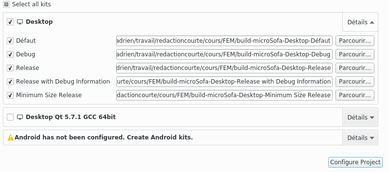
We will now compile the project. For good performance, make sure release mode is selected. If needed, during the lab you can switch to debug mode and use the QtCreator debugger.

The microSofa program takes an argument that is the scene file you want to execute.
In a terminal you can type the following commands:

cd bin
./microSofa default.scn

You can also configure QtCreator to give the path to the scene file parameter (and thus be able to launch the program directly from QtCreator). Go to the Project tab. Select the run mode. Specify in Command line arguments the path to your scene file. (i.e.  microSofaBuild/scene/default.scn).

Press the green arrow in the bottom left to run the program.

During execution you can use the following keys:
    • F1: Displays / Hides the simulation information
    • F2: Displays / Hides the visual mesh
    • F3: Show / Hide fixed points
    • F4: Shows / Hides the Tetrahedric mesh
    • F5: Displays / Hides the mapping
    • F6: Enable / Disable wireframe mode
    • Left Click: Apply a small force on the point under the mouse pointer
    • Right Click: Adds a fixed point constraint to the point under the mouse pointer

Question 1.2: Execute the scene from the previous TP and check that the components you used in Sofa are compatible with the microSofa program. Note: The collisions are not implemented, so it is normal that these components are not created in microSofa. If you do not have these scenes, you can download an implicit and explicit version of the files here. Also, you can refer to this lecture for more information about implicit/explicit time integration.

2) C ++ data structures

The main data structures of the program are described here.

TVec3: A TVec3 is a vector of 3 values describing the x, y, z coordinates for each point of the mechanical problem. For example, you can access the y coordinate of position p with p[1]. The clear function assigns the null vector TVec3(0,0,0). The x, y, and z coordinates will be 0. You will often find std::vector<<TVec3>> i.e. vectors of <TVec3> that can store a list of positions, forces, or velocities. You can access an element of these vectors with the [] operator that returns a TVec3. Therefore, two sets of brackets [][] allow accessing the coordinates. For example, to access the coordinate y of the 3rd point we write: pos[2][1]. The result is then a scalar of type TReal (float or double) according to what is defined in DataStructures).

TMatrixNxN: This type is a matrix representation of data whose size is given by a constant N. You can access the data of a matrix with the [][] operator. The first coordinate gives access to the row data and the second to the column value. For example, you can access row 2 and column 4 of the matrix mat like this: mat[1][3]. You can also multiply matrices and vectors between them with the * operator. For example res=A*b, assign to res the result of the product of matrix A by the vector b.

You can invert a matrix with mat.invert(matInv) function that inverts the matrix mat in matInv. This function returns the mat determinant. This operation is optimized for small arrays (up to 4×4) but is not implemented for larger arrays.

You can initialize a matrix with a set of rows. For example, to initialize the next 3×4 D matrix you can write:

TMat3x4 D(TMat3x4::Line(a,b,c,d),
          TMat3x4::Line(e,f,g,h),
          TMat3x4::Line(i,j,k,l)
);

3) Main Components

The main components are described here. You are asked to open the files at the same time as you read this section, and then to relate the explanations to the source code provided to you.

core / BaseObject:
The BaseObject type is the basic type of the components of the scene graph. All the components that you will use later in your scene file must be inherited from baseObject. A BaseObject allows you to retrieve a pointer to the context with this->getContext(); They also have a Data name that returns the name of the component that was specified in the scene.

core / Factory:
The factory is the component that transforms creates a component whose name is given in the scene file. It contains a list of all the components that can be created from the scene file. To register a new component in the factory you must use the macro DECLARE_CLASS(COMPONENT_NAME) in your cpp file.

Note: There is also a macro DECLARE_ALIAS(NAME_SCENE,CLASS_NAME) which makes it possible to give another name in the file scene than the name of the c ++ class.

core / Data:
The data are the parameters of the components that you describe in your scene file. You can access and edit their value with the getValue and setValue functions. A Data is a c ++ object that is defined as an attribute of a component (in the declaration of the class in the h file). It is templated on the type of parameter (float, double, int string …).

Each Data must be initialized in the constructor of your component, in the order of their declaration in the C ++ class. For example, we initialize the TetrahedronFEMForceField data in its constructor:

TetrahedronFEMForceField::TetrahedronFEMForceField()
: d_youngModulus("youngModulus",100.0,this)
, d_poissonRatio("poissonRatio",0.4,this)
, d_method("method","large",this) {}

Each Data takes parameters with a name (which will be the one used in your scene file), a default value, and the pointer of the component owning the Data (usually this).

core / Context:
The context is an abstraction of a pointer in the scene graph. From a BaseObject, calling this->getContext() the function returns the context of this component (it can be seen as a pointer on the Node). The Context allows to retrieve general parameters of the scene such as the gravity or the time step or the bounding box (see the functions in the source files). More importantly, the context allows to execute visitors with the function processVisitor(Visitor & v)

core / Visitor:
Visitors are c ++ objects that will traverse the graph and apply actions on the components according to their type. A visitor has a function bool processObject(BaseObject *o) that will be called for each object the visitor browses and indicates the processing that the visitor will do. We can then determine the type of the object o with a dynamic_cast in c ++. For example, the following code returns true if and only if the o object is of type Integrator:

The processObject function returns a boolean that indicates whether the visitor should continue or not.

// test if the object is an Integrator
if (Integrator * o = dynamic_cast<Integrator *>(o)) {
  // if yes o is not null then we call the method step
  o->step(0.0001);
}

Visitors are executed from the context. For instance the following code create a VClearVisitor and execute it from the context of the calling component:

// Create a VClearVisitor
VClearVisitor cv(VecID::force);
this->getContext()->processVisitor(vc);

It can also be called directly from the visitor passint the context as parameter:

VClearVisitor (VecID::force).execute(this->getContext());

The processObject function returns a boolean that indicates whether the visitor should continue or not.

Warning: The constructor of the base class Visitor takes an argument m_processChilds parameter to indicate whether the visitor should traverse the subnodes of the graph. This parameter is false by default.

state / State:
The mechanical object gathers the unknowns of your mechanical problem. This is the most important component when you want to recover the forces, positions or velocities of a deformable object. Since many components require access to these data, direct access to the State is possible from the context. So from any component you can recover the MechanicalObject with:

this->getContext()->getMstate();

Access to the data vectors is performed through the mechanism of VecID. A VecID is an identifier that links the name of the desired vector with the data in stored in memory. For example to access the positions of a State one can write:

std::vector<TVec3> & X = m_mstate->get(VecID::position);

The list of VecID is defined in the dataStructures.h file. The State component contains a whole set of functions for performing vector operations.

Question: In the file State.h, implement the following functions to familiarize yourself with the API:
• vClear: Assigns the vector (0,0,0) in all the boxes of the VecID
• vEqBF: Calculate a = b * h
• vPEqBF: Calculates a = a + b * h
• vOp: Calculate res = a + b * h
• vDot: Returns the scalar product of a and b

Each time you implement a function, check that the behavior of the simulation does not change with respect to the binary library provided.

topology / Topology:
The topology component gather the data structures of the mesh. This class is used to return the list of tetrahedra, triangles or textures of the mesh. Direct access to the topology is possible from the Context. So from any component you can retrieve the topology with

this->getContext()->getTopology();

loader / Loader:
Loaders are components that can read a file containing a 3D mesh and then convert it to Sofa Topology. As each type of file (vtk, obj, stl, …) encodes the data in a different way. The loader makes it possible to make the link between these files and a uniform representation of the topology that will be used by the other components.

We will try to implement a loader the VTK mesh that we will name MeshVTKLoader. Create a MeshVTKLoader.h and MeshVTKLoader.cpp file in the loader directory.

Question: Implement the read_vtk_nodes, read_vtk_elements and read_vtk_text methods of the component.

The goal is to read the vtk file given as a parameter in the Data filename and fill in the positions and the geometrical elements (tetrahedra,triangle…) respectively in the MechanicalObject and the Topology.

Open in a text editor the liver_visu.vtk and liver250.vtk files. A VTK file is composed of several sections (the list of points, the list of tetrahedrons or textures …). Each of these sections begins with a heading that describes the type of data in the following file. There is for example a POINTS line which indicates the beginning of the list of the positions of the mesh.

To implement the VTK loader you can copy/past the MeshGmshLoader loader in the loader directory and rename the component to  MeshVTKLoader. The vtk file is parsed by the load method. For than it calls the read_vtk_nodes and read_vtk_elements methods.

The read_vtk_nodes function must read a first integer that indicates the number of points in the list. Then you have to read the data type. For this you can use the following code that will read a string of characters:

std::string type;
in >> type;

Note: the >> operator read a value from the file and convert the result to the type of the given variable. It stops at each space or new line in the file.

Question: Implement the function that reads all the points of the section. For each point you have to read the X, Y and Z coordinates (double) of the point and then add it in the State with the addPoint method.

The read_vtk_elements function must also read a first integer that indicates the number of items in the list. Then, for each element you must read an integer that indicates the type of the element.

• If the type equals 4 the element is a tetrahedron and you must read 4 integers that indicate the indices of the points of the tetrahedron.
• If the type equals 3 then the element is a triangle and you only have to read three integers.

You must then add the item to the Topology to the list of tetrahedra or triangles. It can be done by adding values push_back in the vector:

std::vector<TTetra> & tetras = topo->getTetras();
std::vector<TTriangle> & triangles = topo->getTriangles();

Note: The loader has an attribute d_flipTetra which allows to change the direction of definition of the tetrahedron (direct or indirect). If the VTK file describes the indices a, b, c, d for a tetrahedron you add in the topology the tetrahedron:

• TTetra(a,b,c,d) if d_flipTetra is False
• TTetra(a,b,d,c) if d_flipTetra is True

The read_vtk_tex function will read two integer. Which corresponds to the texture coordinates of the model that needls to be pushed in the vector topo->getTextures().

Question: Implement the above functions.

mapping / Mapping:
The mapping allows to transfer the forces of the mechanical mesh to the visual mesh and vice versa. The mapping components must implement the functions:

    • void apply(): which allows to apply the field of displacement of the mechanical model to the mapped model.
    • void applyJT(TVecID f): which builds a force from the mapped model to the mechanical model.

The init function allows to retrieve a pointer to the m_stateFrom which is the source component (on which the mechanics is computed) of type State whose path is defined by the Data input (by default ".." which means the preceding node); And a second pointer to the m_stateTo which is the target component (visual model or collision) defined by the data output.

We will implement the apply and applyJT functions of BarycentricMapping. This class calculates at initialization two vectors m_map_i and m_map_f. The vector m_map_i[i] gives for the point i of the mapped mesh, the index of the associated tetrahedron in the source topology, while m_map_f[i] returns a vector of 4 double containing the barycentric coordinates of the point in this tetrahedron.

Question: Write the apply() function, which will write the position of the m_stateTo points according to the position of the points in the m_stateFrom and their barycentric coordinates.

Question: Write the applyJT(TVecId vf) function, which express a force defined in the VecID vf of the m_stateTo to an equivalent force on the m_stateFrom in this same VecID.

integrator / Integrator

The integrators make it possible to advance the dynamics of an object by a time step. An integrator implements the method void step (double dt), which will perform the mechanical calculations of FEM meshes contained in the node of the integrator. The dt parameter is the simulation time interval that will elapse after the execution of the step method. In the rest of this TP we will implement an EulerExplicit ingetrator and an EulerImplicit integrator.

animationloop / AnimationLoop

The AnimationLoop component is the first component called by the simulation loop. This component has a single step method, and is mandatory in the scene (if the component is not specified in the scene it will be created automatically).

This component describes the steps that will be performed in one time step. We will implement the DefaultAnimationLoop which only performs a calculation of the deformation of all the FEM models of the scene and then propagates the deformations on the mapped models.

Question: Implement the DefaultAnimationLoop step method. This function will need to achieve two things :

    1) You will need to perform a mechanical calculation step. For that, execute a step of all the integrators of the scene. This can be done by creating your own visitor that will call the step method of all integrators in the scene.
    2) You will need to propagate mechanical model moves to all mapped models. With another visitor you can call the apply method of all mappings in the scene.

To implement points 1 and 2 you have to write your own visitors who will search all the integrators (for step 1) and all the mapping (for step 2) including in the sub nodes of the AnimationLoop.

Note: Remember that the base class of a visitor has an attribute m_processChilds that indicates whether the visitor should browse the child nodes of the context. It must the be specified to true in order to pass through all the component of the scene.

4) Explicit integration

In a first step we will only implement the necessary functions for an explicit integration. Remember that the goal is to solve the equation

where is the mass matrix, the internal forces of the deformable objects that is computed using positions and velocities at the begining of the time step . are the external forces (such as gravity).

constraint / Constraint

The constraints allow to fix points or to impose null displacements. Constraint components must implement the void applyConstraint(TVecID vf) that applies constraints on the vector designed by the VecID f given as parameter.

constraint / BoxConstraint

The component BoxConstraint makes fix the points included in the box d_box. The function d_box.getValue() gives 6 values describing the box with the following meaning X_min Y_min Z_min X_max Y_max Z_max. The indices of points of the mechanical model inside the box are stored in the vector m_indices.

Question: Implement the init() function. The pseudo code is provided in the sources.

Question: Implement void applyConstraint(TVecID vf). This function overwrites the value contained in the VecID  vf passed as a parameter and replaces it with the null vector (0,0,0) for all points that are included in the box. Note that the indices of points are stored in the vector m_indices.

forcefield / forcefield

Forcefield refers to the components that contribute to the internal forces of the mechanical system. A forcefield must implement void addForce(TVecID vf). This function accumulates the internal or external forces in the vector f.

As part of an implicit integration, a Forcefield must also implement the addDforce function that adds the derivatives of the forces. These functions will be studied in the next section (implicit integration).

forcefield / UniformMass

This component add the gravitational forces in the dynamic equation. It is also used to invert the mass matrix (assumed diagonal) in case of an explicit integration. This is done through the addForce and accFromF functions. Implement these functions:

The addForce function applies external forces to the finite element model (in our case, these forces only concern gravity). The function accumulates (in the vector force f passed as a parameter) the gravity force. In order to simplify we consider that all points have the same mass density given by the Data massDensity. Note that the gravity can be obtained from the Context.

The accFromF function solves the linear system . For that, you consider that the matrix is a diagonal matrix whose value are equal to massDensity.

forcefield / TetrahedronFEMForceField

We will implement the TetrahedronFEMForceField functions that apply the internal forces of the model. These forces are given by the non-linear function of the dynamic equation. This function is non-linear since it depends on the positions and velocities.

As explained in lecture, the co-rotational model is a linear model where rotations are added to compensate for geometric nonlinearities. In this lab we will only consider the implementation of the linear version of the ForceField.

Question: The component TetrahedronFEMForceField has a Data method which by default is equal to “large” which correspond to the co-rotational formulation. In order to deactivate the co-rotational formulation specify the method="small" in your scene file and run your own scene again. You should notice that the model should inflate in case of large deformation. This is due to the non linearities, but as a linear model, it is the correct expected behavior that you will implement.

Implementing the init function

The linear model allows to precompute the relation between stresses and displacements, in order to accelerate substantially the computation times of the stiffness matrix at runtime. In particular, this method assembles for each element the local stiffness matrix as follows:

The objective is to fill the vector m_vecKe which is defined as a member of the class. This vector is computed in the init function and should contain for each element the elementary matrix (that is to say that the vector m_vecKe must be resized with the size of the number of elements). Each matrix is a 12×12 matrix. We will detail the computation of matrices (matrix linking constraints to displacements) and of matrix (internal rigidity) in several stages:

Question: Begin by converting the parameters of the FE model (Young’s modulus and Poisson’s ratio) with the traditionally used lamé coefficients (λ and μ) to integrate the finite element method. Here is the lamé coefficient conversion table (source wikipedia). In this table, the Young’s modulus is denoted E and the Poisson’s ratio v. Express λ and μ according to E and v.

Question: Assemble the internal stiffness matrix as following scheme:

We will assume that the model is homogeneous i.e. all elements have the same young modulus and poisson ratio.

Question: We will now build the matrix. This matrix depends on the geometry of the tetrahedron and must be recalculated for each of them. To do this, firstly you will need build the matrix 4X4 as follows:

where x1, y1, z1 are the rest positions of the first point in the tetrahedron. x2, y2, z2 the positions of the second point in the tetrahedron etc. Now solve the following system:

Note that for this, simply inverse . The inverse of noted is a 4×4 matrix that contains all the scalars necessary for the construction of . It is written as follows:

Finally, create the following matrix (6X12):

Question: Assemble the local stiffness matrix for each element . Noticing that the volume of the element Vol_e is calculated from the determinant | | of , assemble as follows:

Note: if the volume is negative, you can add a warning to specify to the user that the tetrahedra are mis-oriented and that you have to change the value of flip_tetra

Implementing the addForce function

The objective of this step is to calculate the contribution of the force on each element (e) on the global mesh of the deformable domain. This step involves calculating the contribution of the internal forces of the volume on the force vector ; Where is the displacement from the initial position.

For this we can assemble the (hollow) matrix K as follows:

is the stiffness matrix (Stiffness) whose dimension is equal to the number of [nb_noeuds * dim] * [nb_noeuds * dim] where dim is the dimension of the problem (2 in 2D, 3 in 3D).

is a globalization matrix that makes it possible to go from the local indication of the element to the global indication of the mesh. It has a single non-zero value (equal to 1) per line / column pair (whose column corresponds to the overall index of the points of the element). This can be schematized in 2D by the following diagram:

Note: To help the readability of this scheme, each cell of represents a sub-matrix of size dim * dim. 0 is the null sub-matrix, and I is the size identity matrix dim * dim. In this example we are in 2D so dim = 2, there are 3 points per element and 6 points in total. is thus a matrix of size [3 * 2] * [6 * 2] that is 6 * 12.

Question 3.6.1: In your report, give the 2D globalization matrix of the triangle defined by the indices [0,5,4].

Question 3.6.2: Give the result of the product of this globalization matrix with the Stiffness matrix of the triangle defined as follows (note that the stiffness matrices are always symmetric):

What do you notice? Explain the usefulness of the globalization matrix? Is it necessary to store it?

The addForce function must multiply the K matrix with the force vector given as a parameter in the function and sum the result in the same vector:

for u you need to take difference between restPosition and position.

Question 3.6.2: implement the addForce function in which you first compute the addKmatrix using a temporary vector.

The matrix is very sparse (which has a lot of 0). This matrix is therefore never stored in a full format. In practice K is only used to produce the product . It will then be necessary to accumulate by element the result of the product:

Note: this matrix is [dof x dim] X [dof x dim] (dim is 2 for 2D and 3 for 3D). each row dimension is dof x dim. if we want to access point marked in red, we can see it is in third row so we have to multiply it with size of row and then plus column.

Question 3.6.2: Implement an implementation in which matrices are stored for each element in the m_vecKe vector. Implement the addForce function in which you will realize the matrix product directly without ever using the global matrix.

Explicit integration

We will now implement the step function of the EulerExplicit. Recall that the principle of implicit integration is to use the positions and speed of the previous time step to update the acceleration of the current time step. The explicit Euler integration is given by the following equations:

Function collects forces applied to the system using only the positions and velocities of the previous time step. From this force, we can deduce the new acceleration and finally integrate successively speeds and positions.

Question: Implement (using the functions that you have written previously) the void function step(double dt) which achieves the integration during a time step dt. For this, the pseudo code is given in the source code.

5) Implicit Integration

We will now implement an implicit integration according to the forward euler format seen in progress. Recall that the principle of temporal integration and solve the equation of the following dynamics:

where is the vector of external forces, is the mass matrix, is the damping matrix and is a nonlinear function that gives the internal forces as a function of a displacement .

In this TP, we will also use the method of mass lumping which consists of distributing the mass only on degrees of freedom. This approximation has the advantage of producing a diagonal matrix . Moreover, in this simplified version, we will consider that all the degrees of freedom have the same mass and therefore all the diagonal elements are equal.

We will also add damping forces on the system. This has the effect of reducing the energy introduced into the integration to stabilize the simulation. This phenomenon can be compared to friction forces for example. In this simplified version, we will use Rayleigh damping. The principle is to apply two numerical factors on mass and rigidity:

where is the damping matrix. α and β can be obtained from the simulation Params and are usually called rayleigh Mass and rayleigh Stiffness.
The implicit Euler integration is very similar to the explicit version, except that the vector is expressed as a function of positions and velocities at the end of the time step.

Since these positions and speeds of t+h are not known, we will consider as a nonlinear function and we will use the Newton-Raphson algorithm to find the equilibrium of the system.
As we have seen in class, we are going to implement a version that achieves only a single iteration of Newton-Raphson. The equation can finally be written as the following function:

This equation implies to derive H with respect to u. In the linear case, we have .

Question: In this TP, we consider that the deformable model follows a linear regime, which means that the internal forces are given by a linear relation of the displacement, and thus can actually be written as , where is a matrix.

Question 4.2.1: Determine the derivative of with respect to u.
To evaluate the right-hand side of the equqation one must be able to implement the product of the derivative of with respect to with a vector, and the product of by a vector.

Question 4.2.2: Implement the addDForce(MechanicalParams params,TVecId vdx,TVecId vdf) function in TetrahedronFEMForceField library, which calculates the product and stores the results in the vector vdx.

About MechanicalParams: In this and the following functions you will use a structure defined in dataStructures.h to extend the functions. The structure contains 3 parameters mfactor, bfactor, kfactor which correspond to the coefficients to multiply with matrix , and . Finally in the integrator component you will need to give values to this structure.

Question 4.2.3: Implement the addDForce(MechanicalParams params,TVecId vdx,TVecId vdf) function in UniformMass library, which calculates the product of the mass matrix (whose diagonal is equal to the mass scalar, as we have used in UniformMass::addForce) and the vector vdf, then stores the result in the vector vdx.

Question 4.2.4: As for explicit integration, write a computeForce function that achieves the right-hand side of the equation (the vector ). You will need to use both the addForce and addDForce functions that you have implemented in the precedent questions.

We must now solve the linear system . The solution of this system is easily obtained by inverting . Nevertheless, is a large matrix whose size is 3n x 3n where n is the number of points of the freedom mesh. Calculating the inverse of this matrix is ​​therefore very difficult in real time. To maintain real-time-compatible performance, the Conjugate Gradient (CG) algorithm will be used to take advantage of the fact that is a defined positive symmetric hollow matrix. These conditions are necessary to guarantee the convergence of the CG. The CG is an iterative algorithm that consists of taking any solution and refining it until it converges on the exact solution. The following peseudo code shows the details of CG and we can see that, to implement a CG, it is necessary to define the multiplication operator of the matrix with a vector.

Question 4.2.5: In the component CGLinearSover, implement a void function mulMatrixVector(TVecId result, TVecId input), which takes a result vector and an input vector. This function carries out the following multiplication:

Question 4.2.6: In the component CGLinearSover, implement a void function solve(TVecId x, TVecId b) that solves the linear system with the CG algorithm. The tolerance and the maximum number of iterations are available with d_tolerance and d_iteration. The CG can be implemented with the pseudo code displayed in precedent question. In this function you will need to use the multiplication operator mulMatrixVector in the previous question and the functions defined in the State library (vEqBF, vqEqBF…).

Question 4.2.7: Update the GUI information assign to m_cg_iter the number of iterations needed to achieve convergence in the CG.

Question 4.2.8: As in explicit integration, implement the void function step(double dt) in which we Integrate positions and speeds over time. To solve the system you will need to replace the solver in explicit version by the CG solver.